Building Robust Predictive Systems for Structured Data

🧑‍💻 Zhipeng “Zippo” He @ School of Information Systems
Queensland University of Technology

• XAMI LAB
• zhipeng.he@hdr.qut.edu.au
• github.com/ZhipengHe
• zhipenghe.me

Comfirmation Seminar
March 15, 2023

Good morning everyone, My name is Zhipeng He and welcome to my comfirmation seminar.

I’m excited to share with you my work on Building Robust Predictive Systems for Structured Data

Supervisory Team

\[ \DeclareMathOperator*{\argmin}{arg\,min} $\newcommand{\one}{\unicode{x1d7d9}}$ "\uD54F" \]

• A/Prof. Chun Ouyang
• Prof. Alistair Barros
• Dr. Catarina Moreira

I’d like to take a moment to acknowledge my supervisory team. They are CHUN, ALISTAIR and Catarina.

Outline

• Research Background
• Research Questions
• Research Plan
• Progress to Date
• Future Work

Let’s start from the background of my research.

Research Background

Let’s start from the background of my research.

Trustworthy AI: Beyond Accuracy

The relation between different aspects of AI trustworthiness (Li et al. 2023).

In current AI research, accuracy is not the only metrics to determine if a model is good or not any more.

The most recent systematic literature review on trustworthy AI provides a big picture of different requirements of achieving trustworthiness.

The performance of models is only one of several important requirements.

Along with performance, robustness is another critical requirement for building trustworthy AI systems.

By improving the robustness, AI systems can be trusted to make decisions with more security.

Robustness in Machine Learning (ML)

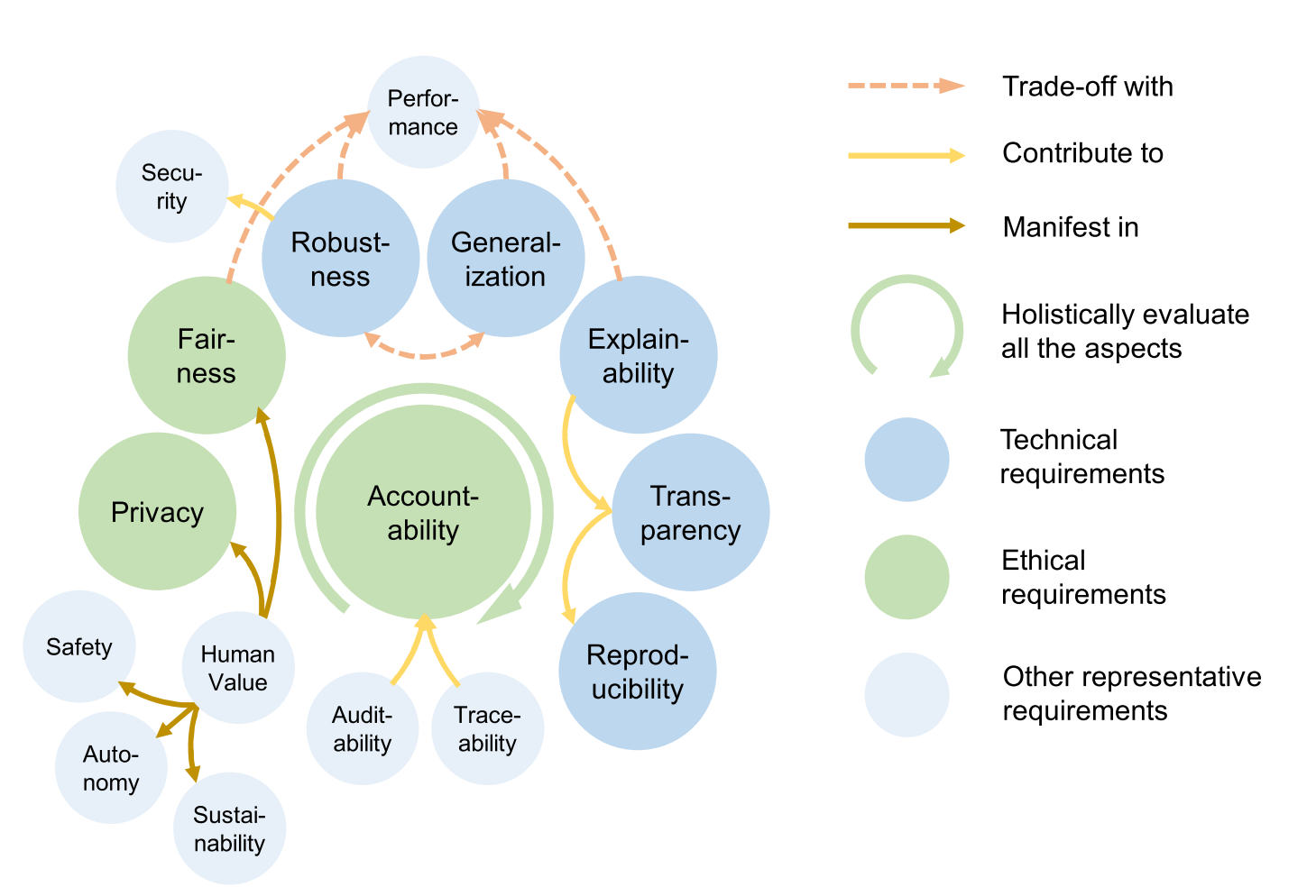
In machine learning, robustness refers to the ability of a model to:

perform well on unseen or new data

variations in the input

A robust model:

• not overly sensitive to perturbation, such as adversarial examples
• generalise enough against distributional variations.

Regarding to the robustness,

In machine learning, robustness refers to the ability of a model to

• perform well on unseen or new data
• particularly for the input variations.

The robustness of model comes from two perspectives:

• not overly sensitive to perturbations, such as adversarial examples
• generalize well against distributional variations.

What are Input Variations?

flowchart LR
  A(Input Variations) --> B(Perturbed Data)
  A --> C(Unperturbed Data)
  B --> D(Adversarial Perturbation)
  B --> E(Non-adversarial Perturbation)
  C --> F(Out-of-distribution)
  C --> G(Outlier & Infrequent Behaviour)
  C --> H(Concept Drift)

Based on these two perspectives, we can categorise the input variations in this figures.

For perturbed data,

• It could be adversarial perturbation, also known as adversarial examples. They are generated by attack algorithms to mislead the predictive models intentionally.

• The other one is non-adversarial perturbation. These variations can be random noise or the input from data augmentation. They usually be used to improve the generalisation of predictive models.

For Unperturbed data, we have

• out-of-distribution data, they have different distribution from trained models.
• outlier data, they usually are extreme value or errors in the input
• Concept Drift, the meaning of target variable in classification problems change over times.

My research will focus on adversarial examples:

• worst-case perturbation,
• if models are robust to adversarial examples it should also be robust to other variations.

Here I will introduce more about the adversarial attacks and examples.

What are Adversarial Attacks?

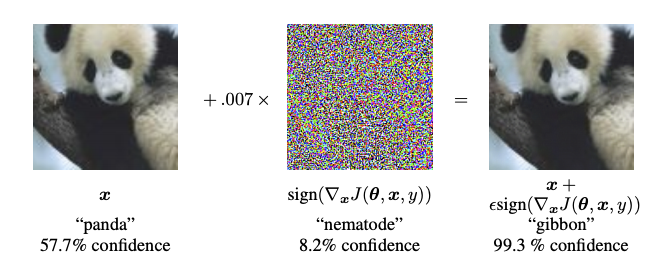
An adversarial attack is a method to generate adversarial examples.

Adversarial examples are specialised inputs created with the purpose of confusing a neural network, resulting in the misclassification of a given input. These notorious inputs are indistinguishable to the human eye but cause the network to fail to identify the contents of the image. (Goodfellow, Shlens, and Szegedy 2015)

let’s understand what are adversarial attack

Shortly, An adversarial attack is a method to generate adversarial examples.

The notion of adversarial examples is defined from two aspects:

• misleading the model predictions
• the perturbation is not noticeable by human eye

For example,

• I have a original image of a panda, and the model predicts it as panda
• after perturbation, the adversarial example is still a panda from human eye.
• However, the predictive model is mislead and output wrong results.

Adversarial Attacks along ML Pipeline

Data Posioning

Backdoor Attack

Evasion Attack

In order to misleading the decision-making of predictive systems, we can use several different methods.

When going through the pipeline of ML. …

• Data poisoning: change the labels in training set
• Backdoor attack: build a predictive model sensitive to specific features
• Evasion attack: use adversarial examples on a trained models

The adversarial attacks will be Evasion attack.

Goal of Adversarial Attacks

Confidence Reduction

Nontargeted Misclassification

Targeted Misclassification

Source/Target Misclassification

Given a credit score classification systems \(f: \mathbb{X}\to \mathbb{Y}\) with three classes \(\mathbb{Y} = \{\)Poor, Standard, Good\(\}\), select an input instance \(\boldsymbol{x}\in\mathbb{X}\) to craft a adversarial example \(\boldsymbol{x}^{adv}\):

1. Attack not success: \(\boldsymbol{x}\) (Poor, 90% confidence) → \(\boldsymbol{x}^{adv}\) (Poor, 50% confidence)
2. Attack success:\(\boldsymbol{x}\) (any class, e.g., Poor) → \(\boldsymbol{x}^{adv}\) (a different class, Standard or Good)
3. Attack success: \(\boldsymbol{x}\) (any class, e.g., Poor or Standard) → \(\boldsymbol{x}^{adv}\) (specific class Good)
4. Attack success:\(\boldsymbol{x}\) (specific class Poor) → \(\boldsymbol{x}^{adv}\) (specific class Good)

After understanding what is adversarial examples and how to use adversarial examples. I’d like to talk about the potential impact after using adversarial examples.

From past literature, they use four goals to describe the impact level of adversarial examples.

Here I use an example to explain the four goals.

There is a credit score classification systems

1. Confidence Reduction: I pick an input from class Poor and the corresponding AE does not flip the prediction, but reduce the confidence
2. Nontargeted Misclassification: I pick an input from any class, e.g., Poor and the AE flips the prediction to the other two classes Standard or Good
3. Targeted Misclassification: i pick an input from any class, e.g., Poor or Standard and I would like make system predict as the specific class Good.
4. Source/Target Misclassification: i pick a input with specific class Poor and I would like make system predict as the specific class Good.

Goal of Adversarial Attacks

Confidence Reduction

Nontargeted Misclassification

Targeted Misclassification

Source/Target Misclassification

Based these understanding, I can rank these four goals by the complexity and difficulty.

Confidence Reduction is easiest and Source/Target Misclassification is hardest.

Adversarial Attack Methods

White-Box Attacks

Grey-Box Attacks

Black-Box Attacks

• Full access to model and dataset knowledge

• Partial access to model and dataset knowledge

• No access to model knowledge; but can query the model

in order to generate adversarial examples, I need to use different types of adversarial attack algorithms.

They are classified into White-Box Attacks, Grey-Box Attacks and Black-Box Attacks.

• White-Box Attacks: Full access to model (parameters and architectures) and dataset knowledge
• Grey-Box Attacks: access to some of model parameters and datasets
• No access to model knowledge; but know the input and output of models.

Adversarial Attack Methods

White-Box Attacks

Grey-Box Attacks

Black-Box Attacks

• FGSM (Goodfellow, Shlens, and Szegedy 2015)
• DeepFool (Moosavi-Dezfooli, Fawzi, and Frossard 2016)

• Not common in practical applications

• Boundary attacks (Brendel et al. 2019)
• Zeroth-order optimisation (Chen et al. 2017)

Here is some methods from each type of attack:

• White-Box Attacks: FGSM and DeepFool
• Grey-Box Attacks: access to some of model parameters and datasets
• Black-Box Attacks: Boundary attacks and Zeroth-order optimisation methods

All these attacks will be measured in my research.

Adversarial Defences

Adversarial defences are techniques used to protect machine learning models from adversarial attacks.

Adversarial Training

Input Randomisation

Defensive Distillation

Ensemble Methods

To improve the robustness of predictive models against adversarial attacks, we can use Adversarial Defences methods

such as:

• Adversarial training: This involves training the machine learning model with adversarial examples during the training phase. The goal is to make the model more robust to future adversarial attacks.
• Input Randomisation: This involves applying transformations to the input data to make it more difficult for an attacker to generate adversarial examples.
• Defensive distillation: This involves training a model to predict the output probabilities of another model. The idea is to make it more difficult for an attacker to generate adversarial examples that can fool both models.
• Ensemble methods: This involves using multiple models to make predictions, with the goal of making it more difficult for an attacker to generate adversarial examples that can fool all the models.

If they have questions:

defensive distillation involves training a single model to predict the output probabilities of another model; Defensive distillation is often used when the original model is particularly important or difficult to replace ensemble methods involve combining the predictions of multiple models; ensemble methods are more flexible and can be used with a variety of models.

Input Data: Image VS Tabular (Mathov et al. 2022)

Image (unstructured):

• High-dimensional
• Homogeneous
• Continuous & consistent features

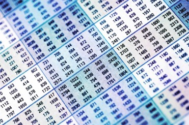
Tabular (structured):

• Low-dimensional
• Heterogeneous
• Numerical & categorical features
• Feature dependencies

In current adversarial machine learning, most of researches work on computer vision. They use unstructured data, such as image to generate adversarial examples.

For image data, it’s:

• High-dimensional
• Homogeneous
• All pixels have same feature range from (0,255)

However, structured data as another important part of data science. It has very different properties than image.

For example, tabular data:

• Low-dimensional
• Heterogeneous
• has both numeric and categorical features, and different feature range
• Feature dependencies from domain knowledge

Due to these differences, when processing tabular data in machine learning, there are lots of challenges

Challenges in Tabular Data (Borisov et al. 2022)

Different feature ranges and feature types

Missing or complex irregular spatial dependencies exist in correlation

Information loss may happen when pre-processing features with dependency

Changing a single feature can entirely flip a prediction on tabular data

• 1The feature ranges are inconsistent and need to deal with both num and cate. features
• 2&3changelings about feature dependencies
• 4 dimentionality: in image chang one pixel will not make effect on prediction, but in tabular..

Sequential Data: Event Log

besides tabular data, there also has sequential data in structured data.

Here gives event logs which is a type of sequential data. event logs record the executions of activities in information systems.

It looks event log as tabular data plus timestamps, but event log is more than a tabular data + timestamp

In this table, each row of table is an activity, it has the information of activity name, time of executions and other features. the case id shows this activity belong to which case.

Because existing of timestamps, we can extract each case as an sequence with order to build a process model. It will make event log more complex than tabular data.

Challenges in Sequential Data

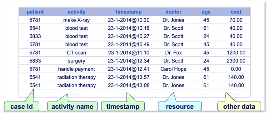
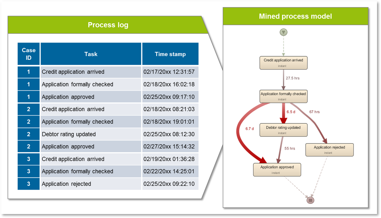
Multi-dimensional feature dependencies

Variable-length inputs

Sequence order constraints

There are also some challengs in processing sequential data

• dependency among features and in the sequence
• the length sequence is differnet for each case
• the order of sequence matters

Current adversarial attacks on Tabular Data

LowProFool attack (Ballet et al. 2019)

• Adapt DeepFool attack into tabular data
• Add feature importance (correlation) to algorithms

Gaps: Only work on numerical features, but not for categorical features.

LowProFool attack is adpated from DeepFool attack for tabular data.

Add feature importance (correlation) to algorithms to determine which feature is important and only change less important features.

However, because it uses feature correlation to calculate the importance. it can only works on numerical features

Current adversarial attacks on Sequential Data (Stevens et al. 2022)

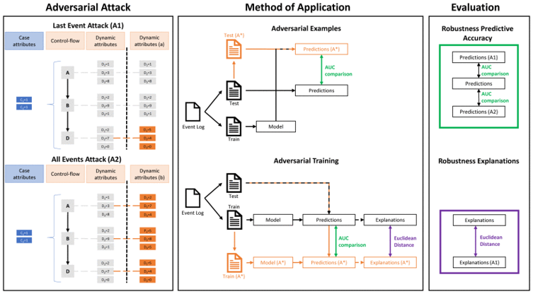
Gaps: Perturb event logs with random noise, but not worst-case perturbation; only perturb dynamic features but not the order of sequence.

Steven’s attack methods attempt to perturb the dynamic features in event logs, for misleading the outcome predictive models.

the underlying concept of the methods is promising, but the approach taken in practice is limited

It only perturb event logs with random noise, but not adversarial examples;

also It only perturb dynamic features but not including the order of sequence.

Research Questions

After the introduce of the adversarial attacks and current gaps in adversarial attacks for strctured data. Here is our research questions

Research Gap & Problem

Researchers have been working on making models more robust to adversarial attacks on unstructured data. However, researchers have rarely investigated adversarial robustness for structured data.

How can one construct predictive models that are robust to adversarial attacks for both tabular data and sequential data?

Most of adversarial machine learning studies work on unstructured data, the adversarial attacks on structured data is under development.

I would like to know “How to build predictive models that are robust to adversarial attacks for both tabular data and sequential data?”

Base on the overall problems, we have three sub questions.

Research Question & Objective 1

RQ1: What characteristics can be applied to determine the success of adversarial attacks on structured data?

RO1: Identify the set of characteristics of successful adversarial attacks on structured data.

The RQ1 is to understand the characteristics of successful adversarial attacks on structured data.

Research Question & Objective 2

RQ2: How to evaluate the characteristics of adversarial attacks (identified in RQ1) on structured data?

RO2: Develop an evaluation framework to benchmark adversarial attacks on structured data.

The RQ2 is to use the characteristics of successful adversarial attacks to evaluate different attack methods.

Research Question & Objective 3

RQ3: What techniques can be utilised to reduce the impact of adversarial attacks, as identified in RQ2, on the robustness of predictive models for structured data?

RO3: Design defence algorithms into predictive models against adversarial attacks for structured data.

The RQ3 is to use the insights from evaluation of different attack methods to help us think of defence methods to improve the robustness.

Research Plan

Based on the research questions,

Research Methodology (Peffers et al. 2007)

I use design science research method to propose a research plan with four phases.

Research Plan

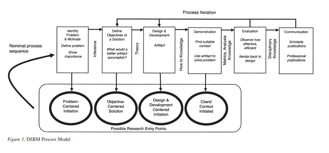
Phase I: Background research, problem definition, and literature review

Phase II: Evaluation of adversarial attack techniques (Iterative)

Phase III: Development and evaluation of defence techniques (Iterative)

Phase IV: Tool implementation and thesis write up

For Phases II and III, I will begin investigation with tabular data and then move on to sequential data.

They are:

Phase I: Background research, problem definition, and literature review

1. Understand the theoretical and experimental background of relevant adversarial attack methods and tools
2. Synthesis characteristics of adversarial attacks from the state-of-the-art literature
3. Identify adversarial attacks and predictive models that are applicable to structured data

In phase I, I explored the research background of adversarial attacks and synthesis characteristics of adversarial attacks for RQ1.

Phase II: Evaluation of adversarial attack techniques (Iterative)

1. Discover and propose metrics for evaluating the characteristics of adversarial attacks identified in Phase I.
2. Develop and apply an evaluation framework for assessing adversarial attacks on structured data .
3. Analyse the evaluation results and derive design mechanisms to design new adversarial attack methods.

In phase II, I proposed research metrics and evaluation framework to evaluate the characteristics of adversarial attacks and analyse the evaluation results

Phase III: Development and evaluation of defence techniques (Iterative)

1. Apply adversarial attack methods in Phase II for adversarial training.
2. Improve and/or re-design adversarial defence techniques for structured data.
3. Evaluate the proposed attack defence techniques using the evaluation framework proposed in Phase II.

In phase III, I will design adversarial attack methods with the insights from Phase II, the designed adversarial attack will be used for adversarial training.

And I will improve and re-design novel adversarial defence methods for structured data. All the defence methods will also be evaluated by the framework in phase 2.

Phase IV: Tool implementation and thesis write up

1. Develop open-source prototypes or frameworks
2. Write the PhD thesis.

In phase IV, I will finish the PhD milestones and deliver the outcomes

Progress to Date

In my last one year research, here is an overview of my current progress

Overall of Progress to Date

• Identify characteristics of adversarial attacks (RQ1)
• Propose evaluation metrics on Effectiveness and Imperceptibility (RQ2)
• Benchmark white-box attack on Effectiveness and Imperceptibility (RQ2)

In my last one year research, here is an overview of my current progress

Completed & In Progress - Identify characteristics of adversarial attacks (RQ1) - Propose evaluation metrics based on characteristics on Effectiveness and Imperceptibility (RQ2) - Benchmark on white-box attack (RQ2)

Future Work

• Extend benchmark evaluation to black-box attack and sequential data (RQ2)
• Improve and/or re-design adversarial defence techniques for structured data (RQ3)

Characteristics of Adversarial Attacks

Phase 1.2

Effectiveness

Imperceptibility

Transferability

• Performance
• Measure the impact on models

• Indistinguishable to human observers
• Assess through knowledge in datasets

• Transfer to other models
• Transfer to other datasets

i identify three Characteristics of adversarial attacks.

The first one is Effectiveness ,also know as performance. the basic Characteristic represents the level of impact on models

The Imperceptibility refer to if the perturbation is easily detected by human observers or not.

Transferability refers to the ability of transfer adversarial examples across different models and datasets. however, because structured data depends on the domain knowledge, it is difficult to transfer between different datasets.

Characteristics of Adversarial Attacks

Phase 1.2

Effectiveness

Imperceptibility

Transferability

I consider the order of three characteristics as following

Effectiveness is the ranking first in all three. it is a requirement of obtaining imperceptibility

imperceptibility will be the second level characteristics

Transferability will be the last level. only a high effective and imperceptible adversarial example will be tested for Transferability on different models.

In the current progress, I have evaluated Effectiveness and imperceptibility. The Transferability will be measured in future work.

Effectiveness Metrics: Accuracy

Phase 2.1

Accuracy drop between Natural Accuracy & Robust Accuracy (Yang et al. 2021).

\[ \begin{gathered} \text{Natural Accuracy}= \frac{1}{n}\sum_{i=1}^{n}\one(f(\boldsymbol{x}_i)=y_i) \\ \text{Robust Accuracy}= \frac{1}{n}\sum_{i=1}^{n}\one(f(\boldsymbol{x}^{adv}_i)= y_i) \end{gathered} \]

The effectiveness is measured by two kinds of metrics.

The first is natural accuracy & Robust Accuracy

natural accuracy: model accuracy without attacks

Robust Accuracy: model accuracy after attacks

Accuracy Drop

Effectiveness Metrics: Success Rate

Phase 2.1

The success rate of an adversarial attack is the percentage of input samples that are successfully manipulated to cause misclassification by the model.

\[ \begin{gathered} \text{Untargeted Success Rate} = \frac{1}{n}\sum_{i=1}^{n}\one( \boldsymbol{x}^{adv})\neq f(\boldsymbol{x}_i)) \\ \text{Targeted Success Rate} = \frac{1}{n}\sum_{i=1}^{n}\one( \boldsymbol{x}^{adv})= y^*_i) \end{gathered} \]

The other one is attack success rate, it measures the percentage of successful adversarial examples in all adversarial examples

Imperceptibility Metrics: Sparsity

Phase 2.1

A good adversarial example is expected to perturb fewer features that will result in changing the model’s prediction.

Here, I adapt \(\ell_0\) norm (Croce and Hein 2019) to tabular data as sparsity metric, which measures the number of changed features in an adversarial example \(\boldsymbol{x}^{adv}\) compared to the original input vector \(\boldsymbol{x}\).

\[ Spa(\boldsymbol{x}^{adv}, \boldsymbol{x})=\ell_0(\boldsymbol{x}^{adv}, \boldsymbol{x})=\sum_{i=1}^{n}\one( x^{adv}_i-x_i) \]

When it comes to Imperceptibility, we proposed metrics from four types of metrics

the first metrics is sparsity. It means …

A good adversarial example is expected to perturb fewer features that will result in changing the model’s prediction. I use L1 norm to measure it.

Imperceptibility Metrics: Proximity

Phase 2.1

A good adversarial example is expected to introduce minimal perturbation, which can be obtained as the smallest distance to the original feature vector.

• \(\ell_p\) norm: common perturbation metrics
• IMAD: adapted from evaluating the quality of counterfactual explanations for tabular data (Mazzine and Martens 2021)

the second metric is Proximity which can be measured by relevant distance metrics

It requires minimal perturbation between attack examples and original inputs

Besides the common Lp norm, I also get inspiration from evaluating the quality of counterfactual explanations for tabular data. and use IMAD distance as another metric

here is the definition of them.

Imperceptibility Metrics: Proximity

Phase 2.1

• \(\ell_1\) norm, which measures the absolute difference. \[ \ell_1(\boldsymbol{x}^{adv}, \boldsymbol{x}) = \sum_{i=1}^n\vert x^{adv}_i- x_i\vert \]

• \(\ell_2\) norm, which measures the square root of the sum of the squared vector values. \[ \ell_2(\boldsymbol{x}^{adv}, \boldsymbol{x}) = \sqrt{\sum_{i=1}^n(x^{adv}_i- x_i)^2} \]

here is the definition of them.

Imperceptibility Metrics: Proximity

Phase 2.1

• \(\ell_\infty\) norm, which measures the maximum difference in feature values. \[ \ell_\infty(\boldsymbol{x}^{adv}, \boldsymbol{x})=\Vert\boldsymbol{x}^{adv}-\boldsymbol{x}\Vert_\infty = \sup_{n}{\vert x^{adv}_n- x_n\vert} \]

• Inverse of median absolute deviation (IMAD), consists of \(\ell_p\) norm normalised by the inverse of the median absolute deviation of feature \(j\) over the dataset. Here we apply \(\ell_1\) norm: \[ \begin{gathered} \text{IMAD}(\boldsymbol{x}^{adv}, \boldsymbol{x})= \sum^n_{i=1}\frac{\vert x^{adv}_i-x_i\vert}{\text{MAD}_i}, \text{where} \\ \text{MAD}_i=\text{med}_{j\in\{1,\cdot,n\}} \vert x_{i,j}-\text{med}_{l\in\{1,\cdot,n\}}(x_l,i)\vert \end{gathered} \]

Inverse of median absolute deviation (IMAD) measures the distance based on the inverse of the median absolute deviation of each feature over the dataset.

Since counterfactual and adversarial examples share the similar underlying concept, they search a nearest datapoint that can flip the prediction, but for different purposes.

Adversarial examples are used to attack and counterfactual examples are used to for explanation.

Imperceptibility Metrics: Distribution

Phase 2.1

Perturbed vectors should be as similarly as possible to the majority of original vectors.

• Mahalanobis distance (MD), which is a multi-dimensional generalization of \(\ell_2\) norm. Given an input vector \(\boldsymbol{x}\), a perturbed vector \(\boldsymbol{x}^{adv}\) and the covariance matrix \(V\), it is defined by: \[ \text{MD}(\boldsymbol{x}^{adv}, \boldsymbol{x})= \sum^n_{i=1}\sqrt{\frac{(x^{adv}_i-x_i)(x^{adv}_i-x_i)^T}{V}} \]

Distribution is the third types of metric for Imperceptibility

The generated adversarial exmaples should be as similarly as possible to the majority of original inputs.

I use MD to measure multi-dimensional generalization of \(\ell_2\) norm

Imperceptibility Metrics: Distribution

Phase 2.1

• Neighbour distance (ND) (Ballet et al. 2019), which computes \(\ell_p\) distance to the closest neighbor \(\boldsymbol{q}\) of original input set \(\mathbb{X}\). Here, I adapt this metric with \(\ell_2\) norm: \[ \text{Neigh}(\boldsymbol{x}^{adv}, \boldsymbol{q}) = \argmin_{\boldsymbol{q}\in \mathbb{X}}\Vert \boldsymbol{x}^{adv}-\boldsymbol{q} \Vert_2 \]

And I use Neighbour distance to computes \(\ell_p\) distance to the nearest neighbor in original dataset

Imperceptibility Metrics: Sensitivity

Phase 2.1

• The notion of perturbation sensitivity for images is calculating the inverse of the standard deviation of the pixel region. (Luo et al. 2018)

• For tabular data, I adapted sensitivity as the inverse of the standard deviation of all numerical features within a set of adversarial examples. \[ \begin{gathered} \text{SDV}(\boldsymbol{x}^{adv})= \frac{1}{n} \sum_{i=1}^n \sqrt{ \frac{ \sum^m ( x^{adv}_{i}- \bar{x}^{adv}_{i})^2 }{ m } }\\ \text{SEN}(\boldsymbol{x}^{adv})=\frac{1}{\text{SDV}(\boldsymbol{x}^{adv})}, \end{gathered} \]

The notion of perturbation sensitivity for images is calculating the inverse of the standard deviation of the pixel region.

For tabular data, we adapted sensitivity as the inverse of the standard deviation of all numerical features within a set of adversarial examples.

Evaluation Framework

Phase 2.2

After establishing the metrics of effectiveness and imperceptibility, I can start the evaluation of these two characteristics.

Here is the overview of my evaluation frameworks.

Firstly, tabular datsets are used to train multiple predictive models.

then, the predictive models are passed to attack methods to generate adversarial examples

At last, adversarial examples will be evaluated from effectiveness and imperceptibility perspectives.

Attack Methods

Phase 1.3 & 2.2

Selection Criteria:

• Applicable to tabular data or sequential data.
• White-box attack.

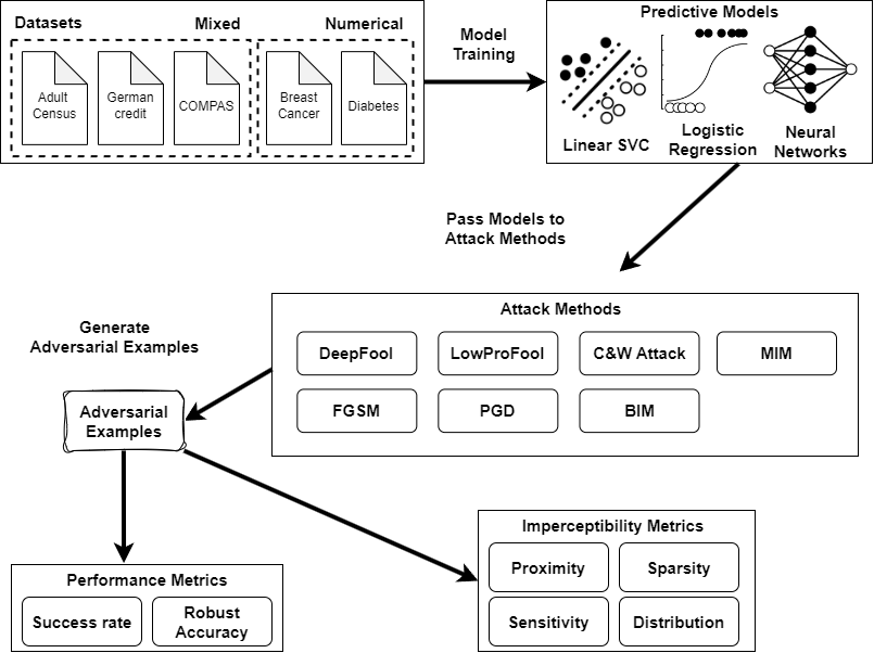
Total 13 variants of 7 attacks with different norm.

Gradient-based: FGSM, BIM, MIM, PGD

Decision boundary-based: DeepFool, LowProFool

Optimization-based: C&W attack

For the implementation details,

The first point is to figure out what attack methods can be used for evaluation.

here I give two criteria, the attack methods must can be used on tabular data or sequential data Second, the current evaluation will focus on white-box attacks.

As a result, a total of 7 attacks were chosen and they can be classified into three groups, based on the underlying differences.

In all 7 attacks, because of different lp norm, there are total 13 variants

Predictive Models

Phase 2.2

Selection Criteria:

• Applicable to tabular data or sequential data.
• At least two attack methods can be applied on the selected model.

Logistic Regression (LR)

Support Vector Machine (SVM)

Multilayer Perceptrons (MLP)

the predictive models in evaluation are required to work on tabular data or sequential data. and At least two attack methods can be applied on the selected model.

We use two transparent machine learning model Logistic Regression (LR) and Support Vector Machine (SVM) and a simple neural network – Multilayer Perceptrons (MLP). To understand the performance of adversarial examples on differnet types of models.

Datasets

Phase 2.2

• UCI Machine Learning Repository
• OpenML-CC18 Benchmarking Suite

Dataset	Data Type	Total Inst.	Train/Test Set	Total Feat.	Cate. Feat.	Num. Feat.	Enc.Cate. Feat.
Adult	Mixed	32651	26048/6513	12	8	4	98
Breast	Num	569	455/114	30	0	30	0
COMPAS	Mixed	7214	5771/1443	11	7	4	19
Diabetes	Num	768	614/154	8	0	8	0
German	Mixed	1000	800/200	20	15	5	58

Five dataset are selected from well-know tabular benchmarking suite

Two of them only have numerical features and the other three of them have both numerical and categorical features.

to deal with categorical features, I use one-hot encoding to transform a categorical feature to a numerical feature space

Model Accuracy

Phase 2.2

Similar and reasonable accuracy among three predictive models suggests comparability of the impact of adversarial examples across models.

Datasets	LR	SVM	MLP
Adult	0.8524	0.8532	0.8521
German	0.8125	0.8125	0.7969
COMPAS	0.7933	0.7976	0.8089
Diabetes	0.7578	0.7578	0.7266
Breast Cancer	0.9844	0.9844	0.9688

After training predictive models, the models’ accuracy are shown here.

For each datasets, the accuracy of three models are similar and reasonable. Hence, I can compare the performance of adversarial attacks across three models.

Finding 1

Phase 2.3

There is a trade-off between imperceptibility and effectiveness.

From the benchmark experiment results, I have derived three interesting findings:

There is a trade-off between imperceptibility and effectiveness.

For example

The following plots show that the Accuracy drop and success rate of FGSM L1 L2 Linf attack is increasing on all five datasets.

L_inf Attack can achieve the most accuarcy drop and almost always achieve 100% success rate. All three models show the same patterns.

However, for imperceptibility, it’s the opposite, the proximity metrics also increase by the order of FGSM L1 -> L2 -> Linf. It represents the decreasing of imperceptibility.

L_inf can only reach the worst imperceptibility. All three models show the same patterns.

Hence, the examples from L_inf attack can be easily picked up.

Finding 2

Phase 2.3

Optimisation-based attacks should be the preferred methods for tabular data.

Overall, C&W \(\ell_2\) attack obtains the best balance between imperceptibility and effectiveness.

C&W attack is designed to optimise a loss function that combines both the perturbation magnitude with distance metrics and the prediction confidence with objective function:

\[ \argmin_{\boldsymbol{x}^{adv}} \Vert\boldsymbol{x}-\boldsymbol{x}^{adv}\Vert_p + c\cdot z(\boldsymbol{x}^{adv}) \]

Optimisation-based attacks should be the preferred methods for tabular data.

Overall, C&W \(\ell_2\) attack obtains the best balance between imperceptibility and effectiveness.

because it treats adversarial attacks as an optimisation problem. It measures both perturbation size and prediction confidence in the loss functions.

Finding 3

Phase 2.3

Adding sparsity as a term in the optimisation function is important for adversarial attacks on structured data.

Adding sparsity as a term in the optimisation function is important for adversarial attacks on structured data.

The experiments show that attack methods tend to change all numerical features.

For example, the two numerical feature only dataset.

Total 8 features in diabetes

Total 30 features in breast cancer

Limitations

Phase 2.3

1. The current metrics are not sufficient for a comprehensive evaluation of successful adversarial attacks.
2. The current encoding methods for categorical features may lead to the high sparsity.

1. The current metrics are not sufficient for a comprehensive evaluation of successful adversarial attacks.

Introduce domain knowledge to the evaluation

2. The current encoding methods for categorical features may lead to the curse of dimensionality.

Future Work

These is the current progress of my research.

For the future, I divide them to three different stage.

Stage 1 of Future Work

Phase 2.1

Introduce domain knowledge into the evaluation of imperceptibility.

Immutability

• Attack methods should not change sensitive features from domain knowledge.

Feasibility

• Attack methods should maintain the soundness of perturbed feature values from domain knowledge.

Stage 1 of Future Work will introduce domain knowledge into evaluation of imperceptibility.

Here I provide two metrics based on domain knowledge, Immutability and Feasibility

:::

Stage 1 of Future Work: Immutability

Phase 2.1

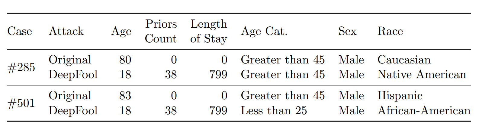
• Likelihood of reoffending are flipped from Medium-Low to High;
• but the feature values of Race are changed.

The present study employs a combination of the COMPAS dataset and a logistic regression model as an example.

In our experiment, all cases were categorised into either ``Medium-Low’’ or High’’ risk categories.

The table showcases two cases (#285 and #501) that were initially predicted as Medium-Low''. The DeepFool attack successfully perturbed these two cases, causing a shift in the decision-making process towardsHigh’’ risk.

However, this perturbation also resulted in a change of race from Caucasian and Hispanic to Native American and African-American.

Stage 1 of Future Work: Feasibility

Phase 2.1

• From medical domain knwoledge, the feasible range of BMI is from 15 (Underweight - Severe thinness) to 40 (Obese Class III).

The diabetes dataset predicts whether a patient has diabetes

We select two cases (#19 and #57) from the diabetes, which original do not have diabetes.

For both Case #19 and Case #57, all three attack methods significantly increase BMI feature from around 30 to greater than 40. It is not feasible given the domain knowledge

Stage 2 of Future Work

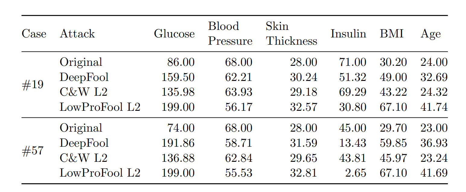
Phase 2.2 & 2.3

Extension of benchmark

• Black-Box Attacks:
  • Bounadry Attack (Brendel et al. 2019)
  • Decision-based Attack (Brendel, Rauber, and Bethge 2018)
  • Zeroth-order Optimisation (Chen et al. 2017)
  • Square Attack (Andriushchenko et al. 2019)
• Tree-based Models & Neural Networks:
  • Decision Tree
  • XGBoost
  • Transformer
  • TabNet
• Sequential Data:
  • Event Logs
  • Sensor Stream
  • Network Traffic Data
  • Time-series Financial Data

Building upon the current design of the evaluation framework, we have successfully assessed the effectiveness and imperceptibility of white-box attacks on tabular data. Moving forward, the next stage of our evaluation process will involve extending the framework to include the following:

Black-box attacks are commonly employed when the attacker lacks full knowledge of the model’s architecture and parameters, or when the model is protected by robust defences that impede the generation of successful adversarial examples using white-box attacks. They are closer to the real-world application and can discover how transferability will affect the adversarial attacks.

the chosen white-box attacks cannot be directly applied to the majority of tree-based predictive models, like XGBoost. By using black-box attacks, the evaluation can also encompass tree-based models and neural networks specifically designed for structured data.

Sequential data is a crucial component of our research scope, and is significantly more complex than tabular data. One of the main challenges in processing sequential data is the need to consider both the temporal ordering of the data points and the interdependence between them, which provides more constraints for the imperceptibility of adversarial examples. Additionally, sequential data often exhibits varying lengths and irregularities, which can pose further difficulties for processing and analysis.

Stage 3 of Future Work

Phase 3

Adversarial Defences

1. Adversarial Training
2. Novel defence mechanisms
3. Ensemble-based approaches

a set of design principles for developing effective adversarial attack and defence algorithms for structured data will be established. Inspired by the concept of adversarial training, we will propose a novel adversarial attack method that generates adversarial examples to be employed in adversarial training as a defence mechanism.

Furthermore, ensemble-based approaches that combine multiple models or defences can also be explored to enhance the overall robustness of the system.

Publication Strategy

1. Imperceptibility Metric & White-box Attack Evaluation on tabular data will be submitted to European Conference on Machine Learning and Principles and Practice of Knowledge Discovery in Databases (ECML PKDD 2023, CORE ranking A) after confirmation seminar.
2. The work on adversarial attack benchmark for tabular data will be submitted to Q1 journal.

Publication Plan

For ECML PKDD, I will submit … in next two weeks

I plan to submit…

We have since taken into account the feedback provided by the reviews and revised the evaluation design accordingly in this report. We intend to resubmit the improved version of our work to European Conference on Machine Learning and Principles and Practice of Knowledge Discovery in Databases (ECML PKDD 2023, CORE ranking A).

Publication Strategy

CORE ranking A* Conferences

• International Joint Conference on Artificial Intelligence (IJCAI)
• Conference on Neural Information Processing Systems (NeurIPS)
• National Conference of the American Association for Artificial Intelligence (AAAI)
• IEEE Symposium on Security and Privacy (SP)

CORE ranking A Conferences

• European Conference on Artificial Intelligence (ECAI)
• European Conference on Machine Learning and Principles and Practice of Knowledge Discovery in Databases (ECML PKDD)
• Pacific-Asia Conference on Knowledge Discovery and Data Mining (PAKDD)
• IEEE International Conference on Data Science and Advanced Analytics (DASS)

Scimago Q1 Journals

• IEEE Transactions on Neural Networks and Learning Systems
• ACM Transactions on Intelligent Systems and Technology
• Knowledge-Based Systems
• Expert Systems with Applications

References

Andriushchenko, Maksym, Francesco Croce, Nicolas Flammarion, and Matthias Hein. 2019. “Square Attack: A Query-Efficient Black-Box Adversarial Attack via Random Search.” arXiv:1912.00049.

Ballet, Vincent, Xavier Renard, Jonathan Aigrain, Thibault Laugel, Pascal Frossard, and Marcin Detyniecki. 2019. “Imperceptible Adversarial Attacks on Tabular Data.” arXiv 1911.03274.

Borisov, Vadim, Tobias Leemann, Kathrin Seßler, Johannes Haug, Martin Pawelczyk, and Gjergji Kasneci. 2022. “Deep Neural Networks and Tabular Data: A Survey.” IEEE Transactions on Neural Networks and Learning Systems.

Brendel, Wieland, Jonas Rauber, and Matthias Bethge. 2018. “Decision-Based Adversarial Attacks: Reliable Attacks Against Black-Box Machine Learning Models.” In 6th International Conference on Learning Representations, ICLR 2018.

Brendel, Wieland, Jonas Rauber, Matthias Kümmerer, Ivan Ustyuzhaninov, and Matthias Bethge. 2019. “Accurate, Reliable and Fast Robustness Evaluation.” arXiv:1907.01003.

Chen, Pin-Yu, Huan Zhang, Yash Sharma, Jinfeng Yi, and Cho-Jui Hsieh. 2017. “ZOO: Zeroth Order Optimization Based Black-Box Attacks to Deep Neural Networks Without Training Substitute Models.” In Proceedings of the 10th ACM Workshop on Artificial Intelligence and Security, AISec@CCS 2017, edited by Bhavani Thuraisingham, Battista Biggio, David Mandell Freeman, Brad Miller, and Arunesh Sinha, 15–26. ACM.

Croce, Francesco, and Matthias Hein. 2019. “Sparse and Imperceivable Adversarial Attacks.” In 2019 IEEE/CVF International Conference on Computer Vision, ICCV 2019, 4723–31.

Goodfellow, Ian J., Jonathon Shlens, and Christian Szegedy. 2015. “Explaining and Harnessing Adversarial Examples.” In 3rd International Conference on Learning Representations, ICLR 2015.

Li, Bo, Peng Qi, Bo Liu, Shuai Di, Jingen Liu, Jiquan Pei, Jinfeng Yi, and Bowen Zhou. 2023. “Trustworthy AI: From Principles to Practices.” ACM Computing Surveys 55 (9): 1–46.

Luo, Bo, Yannan Liu, Lingxiao Wei, and Qiang Xu. 2018. “Towards Imperceptible and Robust Adversarial Example Attacks Against Neural Networks.” In Proceedings of the Thirty-Second AAAI Conference on Artificial Intelligence, (AAAI-18), 1652–59.

Mathov, Yael, Eden Levy, Ziv Katzir, Asaf Shabtai, and Yuval Elovici. 2022. “Not All Datasets Are Born Equal: On Heterogeneous Tabular Data and Adversarial Examples.” Knowl. Based Syst. 242: 108377.

Mazzine, Raphael, and David Martens. 2021. “A Framework and Benchmarking Study for Counterfactual Generating Methods on Tabular Data.” arXiv 2107.04680.

Moosavi-Dezfooli, Seyed-Mohsen, Alhussein Fawzi, and Pascal Frossard. 2016. “DeepFool: A Simple and Accurate Method to Fool Deep Neural Networks.” In 2016 IEEE Conference on Computer Vision and Pattern Recognition, CVPR 2016, 2574–82. IEEE Computer Society.

Peffers, Ken, Tuure Tuunanen, Marcus A. Rothenberger, and Samir Chatterjee. 2007. “A Design Science Research Methodology for Information Systems Research.” Journal of Management Information Systems 24 (3): 45–77.

Stevens, Alexander, Johannes De Smedt, Jari Peeperkorn, and Jochen De Weerdt. 2022. “Assessing the Robustness in Predictive Process Monitoring Through Adversarial Attacks.” In 4th International Conference on Process Mining, ICPM 2022, edited by Andrea Burattin, Artem Polyvyanyy, and Barbara Weber, 56–63. IEEE.

Yang, Shuo, Tianyu Guo, Yunhe Wang, and Chang Xu. 2021. “Adversarial Robustness Through Disentangled Representations.” In Thirty-Fifth AAAI Conference on Artificial Intelligence, AAAI 2021, 3145–53. AAAI Press.

Thank you!

That’s all for my presentation of the confirmation seminar. Thanks for listening.