Building Robust Predictive Systems for Tabular Data and Sequential Data

🧑‍💻 Zhipeng “Zippo” He @ School of Information Systems
Queensland University of Technology

• XAMI LAB
• [email protected]
• github.com/ZhipengHe
• zhipenghe.me

IS Doctoral Consortium 2023
November 23, 2023

Supervisory Team
A/Prof. Chun Ouyang
Prof. Alistair Barros
A/Prof. Catarina Moreira (UTS)

\[ \DeclareMathOperator*{\argmin}{arg\,min} $\newcommand{\one}{\unicode{x1d7d9}}$ "\uD54F" \]

Good morning everyone, My name is Zhipeng He and welcome to my DC presentation.

I’m excited to share with you my work on Building Robust Predictive Systems for Tabular Data and Sequential Data

ML for Tabular & Sequential Data

Machine learning systems for tabular data and sequential data have achieved significant success in various domains, such as loan application processing, health diagnosis, and industrial monitoring.

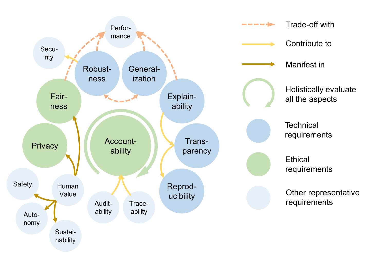
Trustworthy AI: Beyond Accuracy

The relation between different aspects of AI trustworthiness (Li et al. 2023).

Adversarial Robustness

In current AI research, accuracy is not the only metrics to determine if a model is good or not any more.

The performance of models is only one of several important requirements of AI trustworthiness .

Along with performance, robustness is another critical requirement for building trustworthy AI systems.

In our research, we focus on adversarial robustness. It uses adversarial attacks to test the model robustness.

What are Adversarial Attacks?

Adversarial examples are specialised inputs created with the purpose of confusing a neural network, resulting in the misclassification of a given input. These notorious inputs are indistinguishable to the human eye but cause the network to fail to identify the contents of the image. (Goodfellow, Shlens, and Szegedy 2015)

Image Data

Tabular Data

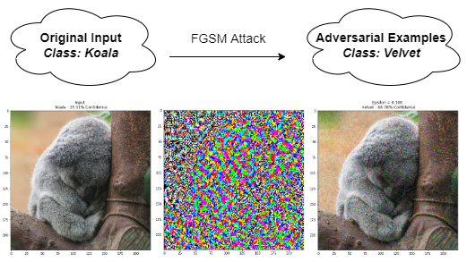
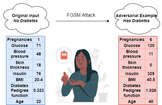
• Mislead the prediction 😊
• Similarity ❓ \(\Longrightarrow\) What makes a good adversarial attack?

let’s understand what are adversarial attack

Shortly, An adversarial attack is a method to generate adversarial examples.

The notion of adversarial examples is defined from two aspects:

• misleading the model predictions
• the perturbation is not noticeable by human eye

For example,

• I have a original image of a koala
• after perturbation, the adversarial example is still a koala from human eye.
• However, the predictive model is mislead and output wrong results.

But when comes to tabular data, things are different I use same Attack algorithm on a case predicting people has diabetes or not?

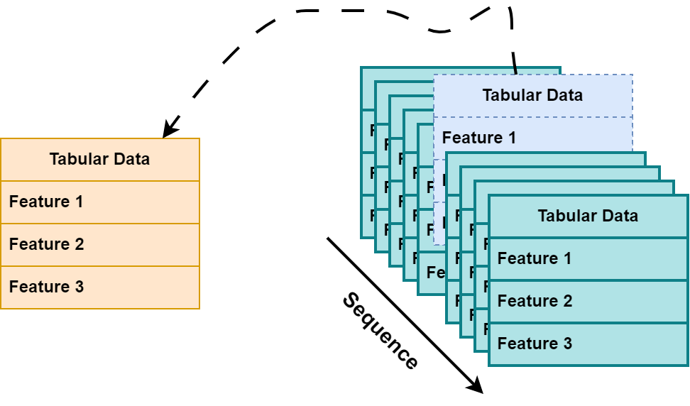
Input Data: Image VS Tabular (Mathov et al. 2022)

Image (unstructured):

• High-dimensional
• Homogeneous
• Continuous & consistent features

Tabular (structured):

• Low-dimensional
• Heterogeneous
• Numerical & categorical features
• Feature dependencies

Look back to data type itself

For image data, it’s:

• High-dimensional
• Homogeneous
• All pixels have same feature range from (0,255)

However, structured data as another important part of data science. It has very different properties than image.

For example, tabular data:

• Low-dimensional
• Heterogeneous
• has both numeric and categorical features, and different feature range
• Feature dependencies from domain knowledge

Due to these differences, when processing tabular data in machine learning, there are lots of challenges

Challenges in Tabular Data (Borisov et al. 2022)

Different feature ranges and feature types

Missing or complex irregular spatial dependencies exist in correlation

Information loss may happen when pre-processing features with dependency

Changing a single feature can entirely flip a prediction on tabular data

• 1The feature ranges are inconsistent and need to deal with both num and cate. features
• 2&3changelings about feature dependencies
• 4 dimentionality: in image chang one pixel will not make effect on prediction, but in tabular..

What Makes A Good Attack

Effectiveness

Imperceptibility

Transferability

• Performance
• Measure the impact on models

• Indistinguishable to human observers
• Assess through knowledge in datasets

• Transfer to other models
• Transfer to other datasets

i identify three Characteristics of adversarial attacks.

The first one is Effectiveness ,also know as performance. the basic Characteristic represents the level of impact on models

The Imperceptibility refer to if the perturbation is easily detected by human observers or not.

Transferability refers to the ability of transfer adversarial examples across different models and datasets.

What Makes A Good Attack

Effectiveness

Imperceptibility

Transferability

I consider the order of three characteristics as following

Effectiveness is the ranking first in all three. it is a requirement of obtaining imperceptibility

imperceptibility will be the second level characteristics

Transferability will be the last level. only a high effective and imperceptible adversarial example will be tested for Transferability on different models.

In our research…

Effectiveness

Imperceptibility

Transferability

• Attack Success Rate

• Sparsity
• Proximity
• Deviation
• Sensitivity
• Fesibility
• Immutability

• Future Work

In our research

The effectiveness are measured by attack success rate

Based on the previous challenges, I obtain six properties for imperceptible adversarial attacks

Each property will be address respectively later.

In the current progress, The Transferability will be measured in future work.

Formalise Adversarial Problems

Given a machine learning classifier \(f: \mathbb{X}\to \mathbb{Y}\) mapping data instance \(\boldsymbol{x} \in \mathbb{X}\) to label \(y \in \mathbb{Y}\), an adversarial example \(\boldsymbol{x}^{adv}\) generated by an attack algorithm is a perturbed input similar to \(\boldsymbol{x}\), where \(\boldsymbol{\delta}\) denotes input perturbation. \[ \boldsymbol{x}^{adv} = \boldsymbol{x} + \boldsymbol{\delta} \hspace{0.8em}\text{subject to } f(\boldsymbol{x}^{adv})\neq y \]

\[Bounded Attack: \max{\mathcal{L}(f(\boldsymbol{x}^{adv}),y)} \hspace{0.8em}\text{subject to } \Vert\boldsymbol{\delta}\Vert \leq \eta \]

\[ Unbounded Attack: \min{\Vert\boldsymbol{\delta}\Vert} \hspace{0.8em}\text{subject to } f(\boldsymbol{x}^{adv})\neq y \]

• Perturbation measured by distance metrics

Before talking about properties of imperceptibility Here gives a mathematical notion of adversarial attacks

By adding perturbation delta, the new generated adversarial example will flip the prediction.

There are two common way to solve the problem, bounded attacks and unbounded attacks

Effectiveness Metrics: Success Rate

The success rate of an adversarial attack is the percentage of input samples that are successfully manipulated to cause misclassification by the model. \[ \text{Attack Success Rate} = \frac{1}{n}\sum_{i=1}^{n}\one( \boldsymbol{x}^{adv}\neq y) \]

The Effectiveness is measured by attack success rate, it evaluates the percentage of successful adversarial examples in all adversarial examples

Imperceptibility Property: Sparsity

A good adversarial example is expected to perturb fewer features that will result in changing the model’s prediction.

Here, I adapt \(\ell_0\) norm (Croce and Hein 2019) to tabular data as sparsity metric, which measures the number of changed features in an adversarial example \(\boldsymbol{x}^{adv}\) compared to the original input vector \(\boldsymbol{x}\).

\[ Spa(\boldsymbol{x}^{adv}, \boldsymbol{x})=\ell_0(\boldsymbol{x}^{adv}, \boldsymbol{x})=\sum_{i=1}^{n}\one( x^{adv}_i-x_i) \]

When it comes to Imperceptibility, we proposed metrics from four types of metrics

the first metrics is sparsity. It means …

A good adversarial example is expected to perturb fewer features that will result in changing the model’s prediction. I use L1 norm to measure it.

Imperceptibility Property: Proximity

A good adversarial example is expected to introduce minimal perturbation, which can be obtained as the smallest distance to the original feature vector.

• \(\ell_p\) norm: common perturbation metrics

\[ \ell_p(\boldsymbol{x}^{adv},\boldsymbol{x})=\Vert\boldsymbol{x}^{adv}-\boldsymbol{x}\Vert_p =\begin{cases} \Bigl(\sum_{i=1}^n(x^{adv}_i-x_i)^p \Bigr)^{1/p}, & p\in\{1,2\}\\ \sup_{n}{\vert x^{adv}_n- x_n\vert}, & p \rightarrow \infty \end{cases} \]

the second metric is Proximity which can be measured by lp distance

It requires minimal perturbation between attack examples and original inputs

here is the definition of them.

Imperceptibility Property: Deviation

Perturbed vectors should be as similarly as possible to the distribution of the original data input.

• Mahalanobis distance (MD), which is a multi-dimensional generalization of \(\ell_2\) norm. Given an input vector \(\boldsymbol{x}\), a perturbed vector \(\boldsymbol{x}^{adv}\) and the covariance matrix \(V\), it is defined by: \[ \text{MD}(\boldsymbol{x}^{adv}, \boldsymbol{x})= \sum^n_{i=1}\sqrt{\frac{(x^{adv}_i-x_i)(x^{adv}_i-x_i)^T}{V}} \]

Distribution is the third types of metric for Imperceptibility

The generated adversarial exmaples should be as similarly as possible to the majority of original inputs.

I use MD to measure multi-dimensional generalization of \(\ell_2\) norm

Imperceptibility Property: Sensitivity

• The notion of perturbation sensitivity for images is calculating the inverse of the standard deviation of the pixel region. (Luo et al. 2018)
• For tabular data, I adapted sensitivity as a normalized \(\ell_1\) distance between \(\boldsymbol{x}\) and \(\boldsymbol{x}^{adv}\) by the inverse of the standard deviation of all numerical features within the input dataset \(\mathbb{X}\).

\[ \begin{gathered} \text{std}(\boldsymbol{x}^{adv})= \sqrt{ \frac{ \sum^m ( x_{i}- \bar{x}_{i})^2 }{ m } }\\ \text{sen}(\boldsymbol{x}^{adv})=\frac{\vert x^{adv}_{i} - x_{i} \vert}{\text{std}(\boldsymbol{x}^{adv})}, \end{gathered} \]

The notion of perturbation sensitivity is adapted from image.

We use l1 by the inverse of the standard deviation of all numerical features to calculate the sensitivity.

Imperceptibility Property

Introduce domain knowledge into the evaluation of imperceptibility.

Immutability

• Attack methods should not change sensitive features from domain knowledge.

Feasibility

• Attack methods should maintain the soundness of perturbed feature values from domain knowledge.

For tabular data, we also want to introduce domain knowledge into evaluation of imperceptibility.

Here I provide two metrics based on domain knowledge, Immutability and Feasibility

These two properties will be assessed by case-based qualitative study

:::

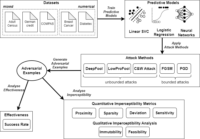
Experiment Pipeline

After establishing the metrics of effectiveness and imperceptibility, I can start the evaluation of these two characteristics.

Here is the overview of my evaluation frameworks.

Firstly, tabular datsets are used to train multiple predictive models.

then, the predictive models are passed to attack methods to generate adversarial examples

At last, adversarial examples will be evaluated from effectiveness and imperceptibility perspectives.

Model Accuracy

Similar and reasonable accuracy among three predictive models suggests comparability of the impact of adversarial examples across models.

Datasets	LR	SVM	MLP
Adult	0.8524	0.8532	0.8521
German	0.8125	0.8125	0.7969
COMPAS	0.7933	0.7976	0.8089
Diabetes	0.7578	0.7578	0.7266
Breast Cancer	0.9844	0.9844	0.9688

After training predictive models, the models’ accuracy are shown here.

For each dataset, the accuracy of three models are similar and reasonable. Hence, I can compare the performance of adversarial attacks across three models.

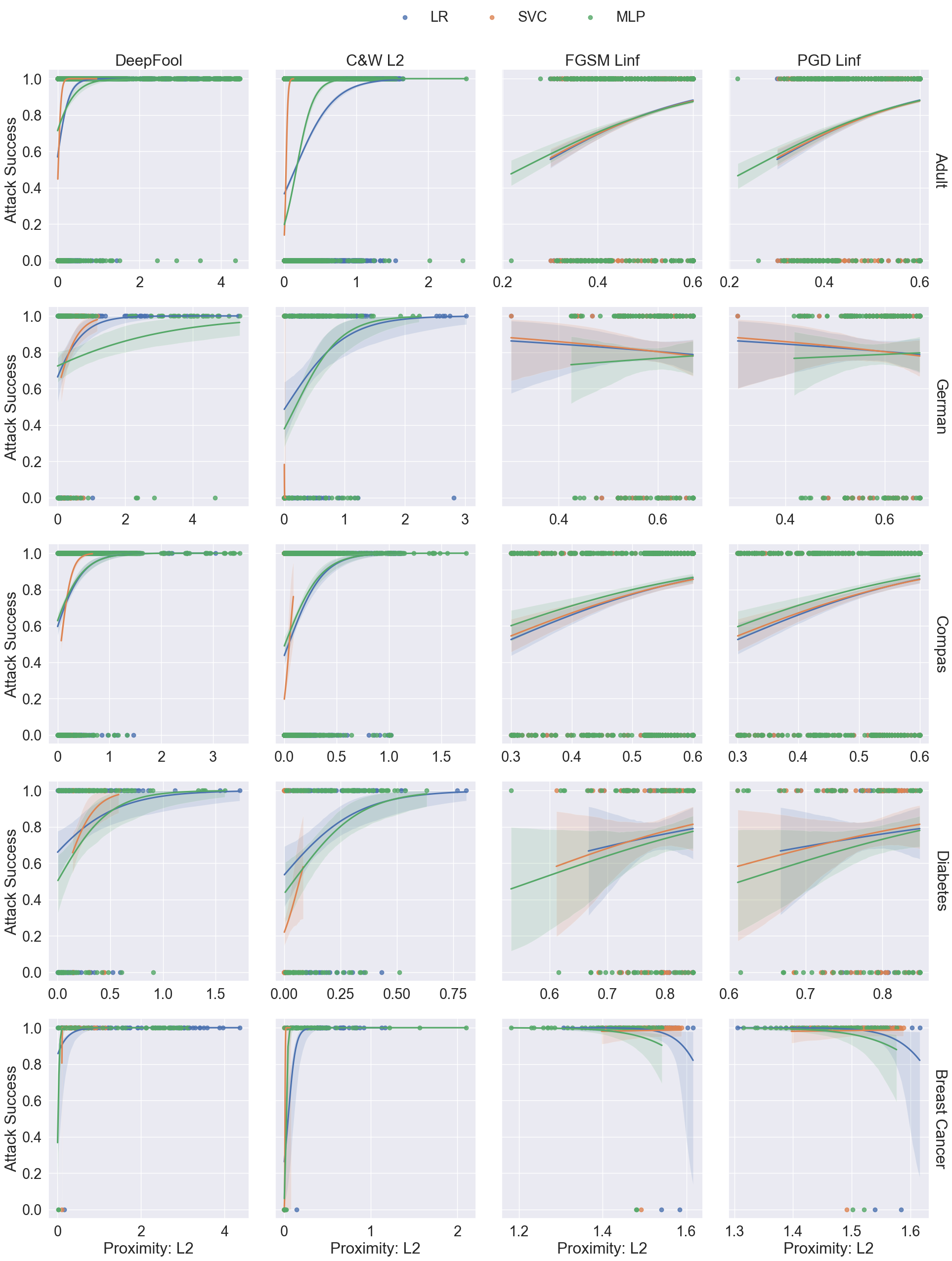
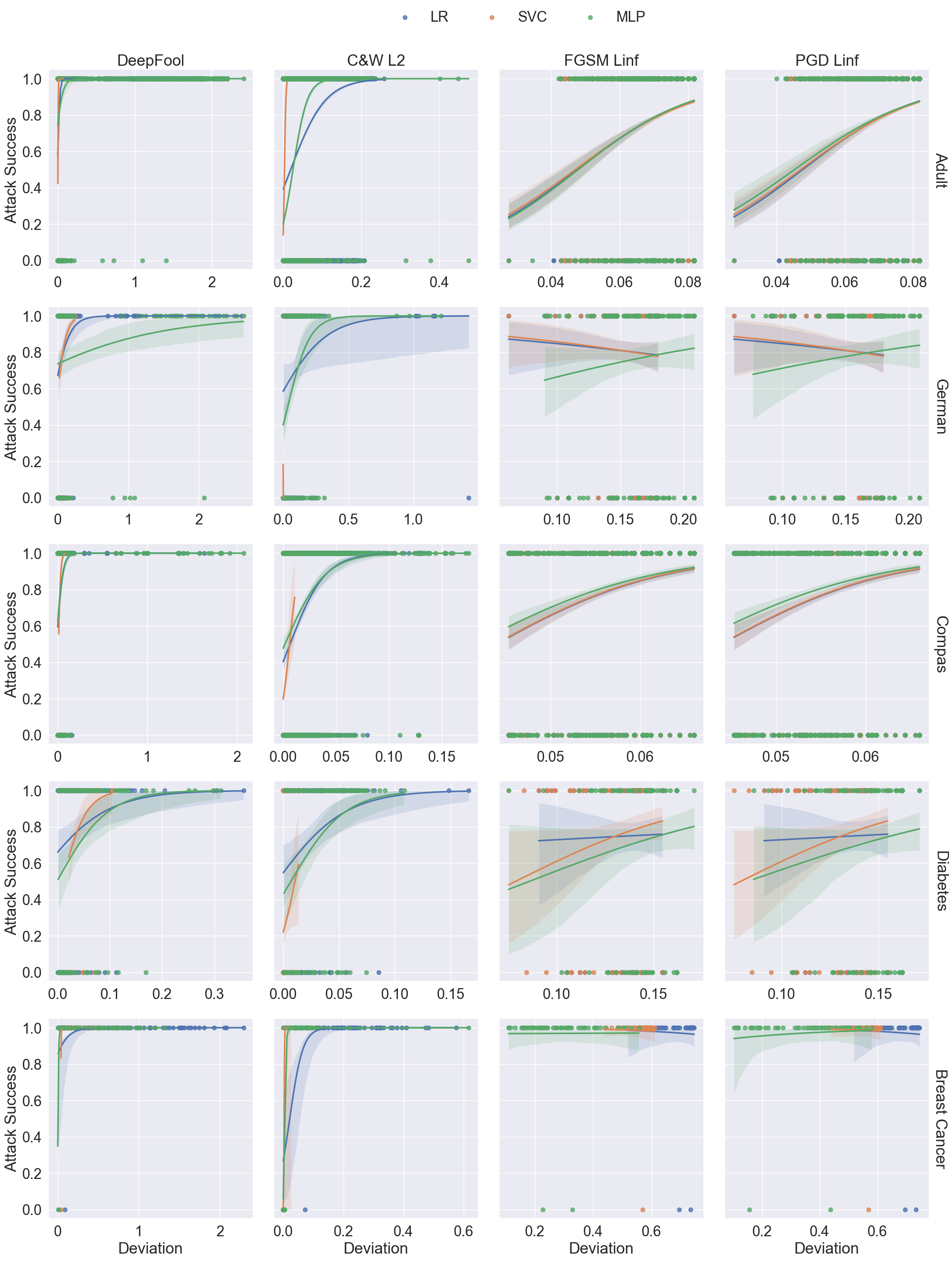
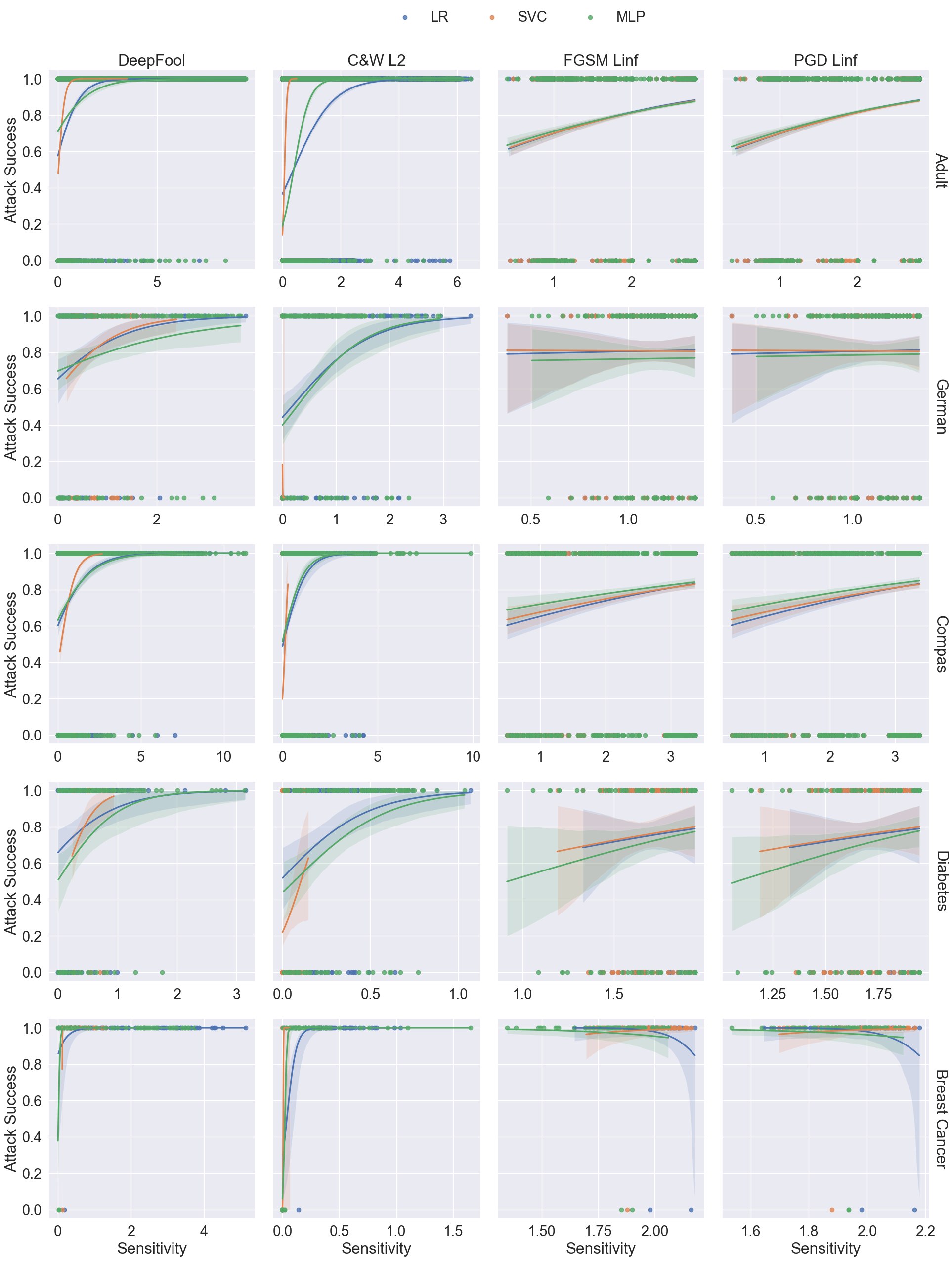
Finding 1

Phase 2.3

There is a trade-off between imperceptibility and effectiveness.

From the benchmark experiment results, I have derived three interesting findings:

There is a trade-off between imperceptibility and effectiveness.

For example

The following plots show that the Accuracy drop and success rate of FGSM L1 L2 Linf attack is increasing on all five datasets.

L_inf Attack can achieve the most accuarcy drop and almost always achieve 100% success rate. All three models show the same patterns.

However, for imperceptibility, it’s the opposite, the proximity metrics also increase by the order of FGSM L1 -> L2 -> Linf. It represents the decreasing of imperceptibility.

L_inf can only reach the worst imperceptibility. All three models show the same patterns.

Hence, the examples from L_inf attack can be easily picked up.

Finding 2

Optimisation-based attacks should be the preferred methods for tabular data.

Overall, C&W \(\ell_2\) attack obtains the best balance between imperceptibility and effectiveness.

C&W attack is designed to optimise a loss function that combines both the perturbation magnitude with distance metrics and the prediction confidence with objective function:

\[ \argmin_{\boldsymbol{x}^{adv}} \Vert\boldsymbol{x}-\boldsymbol{x}^{adv}\Vert_p + c\cdot z(\boldsymbol{x}^{adv}) \]

Optimisation-based attacks should be the preferred methods for tabular data.

Overall, C&W \(\ell_2\) attack obtains the best balance between imperceptibility and effectiveness.

because it treats adversarial attacks as an optimisation problem. It measures both perturbation size and prediction confidence in the loss functions.

Finding 3

Adding sparsity as a term in the optimisation function is important for adversarial attacks on structured data.

Adding sparsity as a term in the optimisation function is important for adversarial attacks on structured data.

The experiments show that attack methods tend to change all numerical features.

For example, the two numerical feature only dataset.

Total 8 features in diabetes

Total 30 features in breast cancer

Qualitative Analysis: Immutability

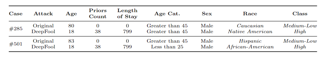
• Likelihood of reoffending are flipped from Medium-Low to High;
• but the feature values of Race are changed.

For immutability and feasibility, case-based study are used to evaluate them

The DeepFool attack successfully perturbed these two cases, causing a shift in the decision-making process towards ``High’’ risk.

However, this perturbation also resulted in a change of race from Caucasian and Hispanic to Native American and African-American.

From the LR feature importance, race feature has negative contribution to prediction.

Qualitative Analysis: Feasibility

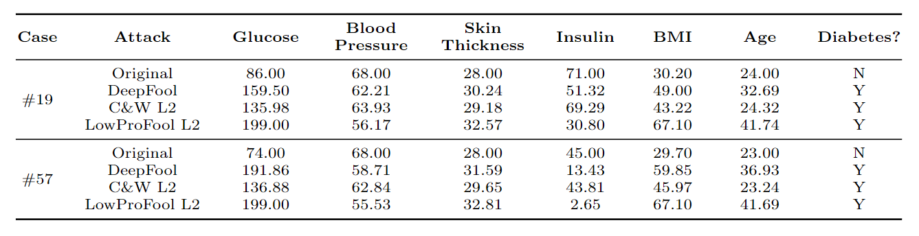
• From medical domain knwoledge, the feasible range of BMI is from 15 (Underweight - Severe thinness) to 40 (Obese Class III).

The diabetes dataset predicts whether a patient has diabetes

All three attack methods significantly increase BMI feature out of the feasible range of BMI

Limitations

• Limitations in evaluation settings
  • Fixed perturbation budget \(\eta=0.3\)
  • Limited num of datasets, models & attacks
• Side effects of one-hot encoding
  • Categorical features similarity measure:
    • Gower’s Distance (Gower 1971)
    • Modified Value Difference Metric (Cost and Salzberg 1993)
    • Association-Based Distance Metric (Le and Ho 2005)
• Absence of ablation study for tabular data

1. We do not have a very comperhensive evaluation

2. We use one-hot encoding for categorical feature to use distance metrics But they actually have own similarity measure

3. We do not perform ablation study

Future Work

Considering my research topic and current progress, we will extend our research to sequential data. Due to the relationship between tabular data and sequential data, some more interesting work can be done in future.

References

Borisov, Vadim, Tobias Leemann, Kathrin Seßler, Johannes Haug, Martin Pawelczyk, and Gjergji Kasneci. 2022. “Deep Neural Networks and Tabular Data: A Survey.” IEEE Transactions on Neural Networks and Learning Systems.

Cost, Scott, and Steven Salzberg. 1993. “A Weighted Nearest Neighbor Algorithm for Learning with Symbolic Features.” Machine Learning 10: 57–78.

Croce, Francesco, and Matthias Hein. 2019. “Sparse and Imperceivable Adversarial Attacks.” In 2019 IEEE/CVF International Conference on Computer Vision, ICCV 2019, 4723–31.

Goodfellow, Ian J., Jonathon Shlens, and Christian Szegedy. 2015. “Explaining and Harnessing Adversarial Examples.” In 3rd International Conference on Learning Representations, ICLR 2015.

Gower, John C. 1971. “A General Coefficient of Similarity and Some of Its Properties.” Biometrics, 857–71.

Le, Si Quang, and Tu Bao Ho. 2005. “An Association-Based Dissimilarity Measure for Categorical Data.” Pattern Recognition Letters 26 (16): 2549–57.

Li, Bo, Peng Qi, Bo Liu, Shuai Di, Jingen Liu, Jiquan Pei, Jinfeng Yi, and Bowen Zhou. 2023. “Trustworthy AI: From Principles to Practices.” ACM Computing Surveys 55 (9): 1–46.

Luo, Bo, Yannan Liu, Lingxiao Wei, and Qiang Xu. 2018. “Towards Imperceptible and Robust Adversarial Example Attacks Against Neural Networks.” In Proceedings of the Thirty-Second AAAI Conference on Artificial Intelligence, (AAAI-18), 1652–59.

Mathov, Yael, Eden Levy, Ziv Katzir, Asaf Shabtai, and Yuval Elovici. 2022. “Not All Datasets Are Born Equal: On Heterogeneous Tabular Data and Adversarial Examples.” Knowl. Based Syst. 242: 108377.

Thank you!

• github.com/ZhipengHe/Imperceptibility-in-Adversarial-attack
• slides.zhipenghe.me/2023-IS-DC
• with by Zhipeng “Zippo” HE with Reveal.js & Quarto